
In the world of statistics and machine learning, Mean Squared Error (MSE) is a fundamental metric used to quantify the accuracy of a predictive model. This article aims to explain the fundamentals of MSE, starting with its definition and delving into its applications, advantages, and limitations. We’ll explore practical examples and demonstrate how to calculate MSE using Python and R to provide a comprehensive understanding of this crucial metric.
What is Mean Squared Error?
Mean Squared Error (MSE) is a statistical measure that quantifies the average squared difference between predicted values and actual values in a regression model. In other words, it assesses how well a model’s predictions align with the observed data by computing the average of the squared differences between predicted and actual values.
Mathematically, MSE is defined as:
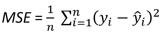
where n is the number of observations, yi represents the actual values, and ŷi represents the predicted values.
When to Use Mean Squared Error
MSE is particularly useful in scenarios where the magnitude of prediction errors is crucial. Here are some instances where MSE is commonly employed:
- Regression Models Evaluation: MSE is widely used to evaluate the performance of regression models. It provides a quantitative measure of how well the model predicts the outcome variable.
- Loss Function in Optimization: MSE is often employed as a loss function during the training of machine learning models. Minimizing the MSE during training helps improve the model’s ability to make accurate predictions.
- Homoscedasticity Assessment: MSE can be used to assess homoscedasticity, a key assumption in regression analysis. Homoscedasticity implies that the variance of the errors is constant across all levels of the independent variable.
Pros and Cons of Mean Squared Error
Pros:
- Sensitivity to Deviations: MSE penalizes larger errors more heavily than smaller ones, making it sensitive to significant deviations between predicted and actual values.
- Well-Defined Mathematical Formulation: The mathematical formulation of MSE is straightforward, making it easy to interpret and implement.
- Differentiable Property: The differentiability of the MSE function is beneficial for optimization algorithms during model training.
Cons:
- Sensitivity to Outliers: MSE is highly sensitive to outliers, as squaring the errors amplifies their impact on the overall metric.
- Assumption of Homoscedasticity: MSE assumes homoscedasticity, meaning that the variance of the errors is constant across all levels of the independent variable. If this assumption is violated, MSE may not accurately reflect model performance.
- Bias Towards Models with Smaller Errors: MSE tends to give more weight to models that exhibit smaller errors, potentially neglecting other important aspects of model performance.
Calculating Mean Squared Error: Python and R Examples
Let’s delve into practical examples to illustrate how MSE is calculated using both Python and R.
Python code example:

# Importing necessary libraries
from sklearn.metrics import mean_squared_error
import numpy as np

# Generating sample data
np.random.seed(42)
actual_values = np.random.randint(0, 100, 50)
predicted_values = actual_values + np.random.normal(0, 10, 50)

# Calculating Mean Squared Error
mse = mean_squared_error(actual_values, predicted_values)

print(f'Mean Squared Error: {mse}')
R code example:

# Generating sample data
set.seed(42)
actual_values <- sample(0:100, 50, replace = TRUE)
predicted_values <- actual_values + rnorm(50, 0, 10)

# Calculating Mean Squared Error
mse <- mean((actual_values - predicted_values)^2)

cat('Mean Squared Error:', mse, '\n')
To show this in action further you can click the button below to see a random dataset be generated and the MSE calculated from it:
As displayed, there are 10 random examples provided here. By choosing prediction numbers at random (whereas you would presumably use numbers received from a predictive model) I can calculate the differences between each value, squared. By taking the average of all the results in each step, I wind up with the desired MSE for the set. Feel free to click the MSE button again to see different examples and predictive values.
Hopefully this demonstration proves that the scary-looking mathematical model from earlier isn't really that complex to use in real life!
Example Scenarios
Let's consider two scenarios to demonstrate the application of Mean Squared Error.
Scenario 1: Housing Price Prediction
Imagine you are developing a model to predict housing prices based on various features such as square footage, number of bedrooms, and location. After training the model, you use MSE to evaluate its accuracy by comparing predicted and actual housing prices for a test dataset.
Scenario 2: Stock Price Forecasting
In the financial domain, suppose you are building a model to forecast stock prices. MSE can help you assess how well your model predicts future stock prices by quantifying the squared differences between predicted and actual stock values.
Mean Squared Error is a valuable metric for assessing the accuracy of predictive models, particularly in regression analysis. Its sensitivity to deviations and well-defined mathematical formulation make it a popular choice in various fields. However, practitioners must be aware of its limitations, such as sensitivity to outliers and the assumption of homoscedasticity.
By understanding MSE and its applications, analysts and data scientists can make informed decisions when evaluating and fine-tuning regression models. The provided Python and R examples offer practical insights into calculating MSE, enabling you to implement and interpret this metric in your own data analysis and machine learning projects.
Comments are closed.