Predicting the price of housing at any given moment in time is highly desirable for a multitude of reasons. By augmenting the forecasting side of things and observing the impact features have upon a house price, better predictions should follow. The aim is to combine both ideas; understand the price of a home given its features and to understand the impact of money through time (think, inflation).
This post is the second part of an analysis I performed on housing features and their impact to prices. In the previous post I walked through how to clean the datasets in Python and set everything up for acceptance in a machine learning model. I am excited to share the results of all that effort!
Resources
Before jumping into the regression model it would be good to read through the preprocessing steps in the previous post. In addition to that, the Python script for this regression model is available on my GitHub. As a refresher, the Kaggle competition has the rules of the analysis and datasets that I leveraged for this project. The following analysis will make a lot more sense after being familiar with the background, but I still walk through every step individually as I go.
Setting Up the Model
Picking up where preprocessing ended, the first item on the agenda is to set up the data for ingestion. There are three distinct arrays that scikit-learn needs in order to get the results needed here:
- Testing Features: we need an array of all the testing features created (294 to be exact) to pass into a trained model
- Training Features: just like with testing, we need an array specifically encompassing all training data
- Training Target: an array is needed for the target of the analysis; for this project, that would be the sale price
All three of these are accomplished through the following code:
x_test = df_testing.iloc[:,:].values
x_train = df_training.iloc[:,0:-1].values
y_train = df_training.iloc[:,-1].values
With these in place, the next step is to set up the linear regression model:
lin = sklearn.linear_model.LinearRegression()
lin.fit(x_train,y_train)
In the last line I fit the linear model to the training features (x_train) and sale price (y_train) distinctly. This is where scikit-learn takes the information and runs the regression against all the data created in the preprocessing step. Once completed, I can use the model to predict any sales price I want given that I pass the same parameters (number of features) to this model. The syntax for prediction is lin.predict() and it is covered next.
Predicting the Testing Dataset
The purpose of this project is to create a model that can predict the testing data features with as high of accuracy as possible. The heart of the Python code is below for validating everything done so far:
testPrediction = lin.predict(x_test)
TestingPrediction = []
for i in testPrediction:
    x = round(i,0)
    TestingPrediction.append(x)
# add prediction and ids to testing dataset
y_export = pd.DataFrame(TestingPrediction)
y_export.columns=['Prediction']
df_testing['Prediction'] = TestingPrediction
df_testing['Id'] = testingIDs
Let’s walk through everything going on here.
First, I create an array that gets assigned to ‘testPrediction’. The lin.predict(x_test) code is where the linear regression model is applied to the testing dataset. At this point I do not know how well my model is performing as that will be assessed when my results get uploaded to Kaggle.
Second, the code that follows passes the sale price predictions of my testing dataset to a list. I use the for loop to accomplish this and then append that list to the original testing dataset. Lastly, I go ahead and reattach the testing IDs to the testing dataset so that I can parse them off later for analysis.
Assessing Model Success
The code in the Python script which follows the regression test is done against the testing dataset. I will not post that again given that it performs the same task except it applies predictions to the training dataframe. With that completed, I can now run a few measurements to get a sense of how well the regression model behaves against home sales prices that we know.
R2, Mean Squared Error (MSE) and Root MSE
The R2 value on a regression model gives a good indication of variance between the dependent and independent variables. A number that is at or close to zero indicates no correlation while one close to one indicates strong correlation. Getting exactly one for R2 would indicate perfect correlation; certainly that is something not to be realistically expected on real-world data.
To get the R2 value from this regression model I executed the following code:
r2 = round(lin.score(x_train,y_train),4)
print('\nR2 Value:',r2)
This yields a value of 93.14%; very good! This shows me that we have a set of features that is strongly predicting the sale price of the house; in other words, there is correlation between dependent/independent variables.
Next, I can run the following to asses the MSE and RMSE of the model:
# mean-squared error
mse = round(mean_squared_error(y_true=df_rmse['SaleLog'],y_pred=df_rmse['PredictionLog']),4)
print('\n')
print('MSE:',mse)
# root mean-squared error
rmse = round(np.sqrt(mse),4)
print('RMSE:',rmse)
The results are 0.0124 and 0.1114, respectively. Again, another great result! This means that the distances between the actual and estimated values are consistently pretty low. Judging by the result I received from the Kaggle competition on my test predictions, this is in the top 25% of models as of the date of this post!
Visualization Analysis
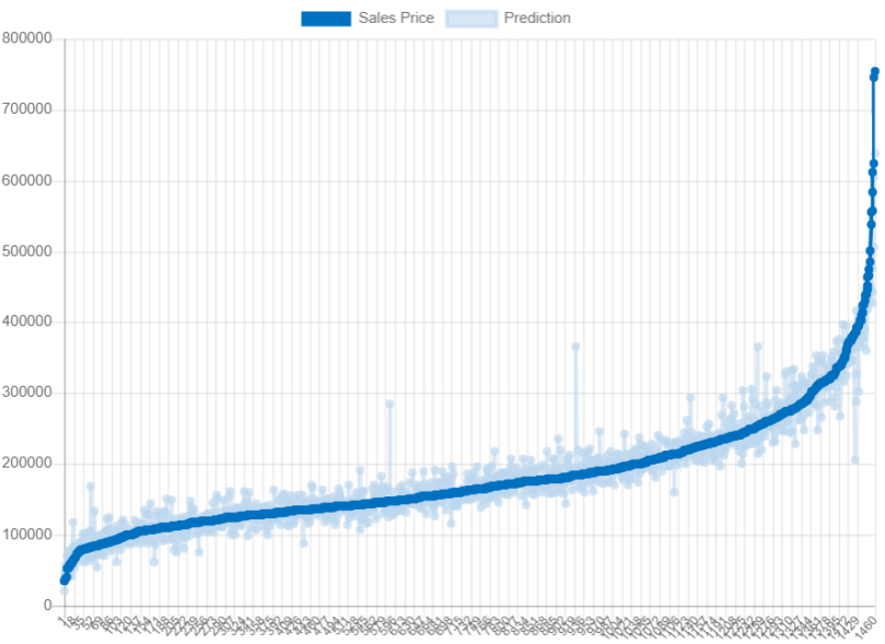
Viewing this data visually is equally insightful in seeing how well our predictions really were. The following displays the actuals vs. estimates on the training set. You can click on the headers in the legend to display or remove data:
What I like about visualizing the model in this way is the beautiful sale price line going directly through the middle of the predictions. This is a great way to think of regression models in fitting the best line for the data. Additionally, knowing that we are dealing with a good-sized regression model makes it even more impressive. A typical regression line will be linear and straight, however, in this case the line can go in many directions. That is because we have a good amount of coefficients contributing to the model and its complexity, but clearly, the results prove it’s worth the effort.
Ending Analysis & Conclusions
As mentioned already, as of the writing of this post my model placed in the top 25% of entrants. Given that this was my first formal competition on Kaggle I am humbly proud. Additionally, I could have done even better if I hadn’t rounded my prediction results on the testing set, but I felt it was the best way to post the data.
The other thing I could have done is to execute more complicated regression models for better results. Gradient boosting is one that comes to mind among others. However, since I am happy with my results for this competition I decided to reserve those methods for another time.
For me, the big deal here was the feature engineering (covered in the previous post) using OneHotEncoder. I have always kind of feared using it and felt that it would take a lot of work to execute. While this wasn’t entirely untrue, the loop I made to automatically create and attach new columns to the dataset makes it reusable code. Therefore, I should be able to comfortably use it on other projects going forward…and you can use it too!
Overall, I think this was a very fun project and well worth the effort I put in. Developing new code and using data I’d never seen before was excellent to learn from. It is also empowering to see that my results held up to scrutiny and I had a strong standing against many others. I know how I could improve the model and as I take on new projects I will go deeper and deeper into new approaches. I am really looking forward to the next project!
This wraps up both articles on housing prices and how I was able to use preexisting data to predict values on any variable. Thanks for reading and I hope this project provided some insight and assistance in understanding machine learning, Python and my thought processes.
Good luck on your future projects!