Housing Cost: Data Model

Housing prices seem to be one of those topics that comes up almost daily. The discussion is either coming from the news, social media, friends, family or just meandering somewhere in the back of people’s minds. This makes sense of course since housing is one of the most sought-after and necessary parts of a healthy life. As I assume everyone does, I couldn’t help but wonder if housing cost is something that machine learning could predict. I mean, who doesn’t sit around and think of everything through the lens of analysis, statistics and machine learning?

With this on my mind, I figured I would go out and find some publicly available data and see if I could take a shot at housing prices. Very quickly, I came upon this wonderful competition from Kaggle which sought to challenge people to predict exactly this! If you are not aware, Kaggle is known for doing many of these types of competitions and they have some good datasets to go along with it.

Having never dug into the website that much in the past, this time I decided to take a shot at it. I figured I could take on some different concepts I haven’t yet in machine learning, primarily feature engineering. This particular project had a good amount of it and was very fun to work on!

This post and the next are a walkthrough of my starting point, data cleanup, and final results. In this initial post I will dive pretty heavy into Python and conduct a lot of code-walking. If the final result is of more interest to you then check out the next post on running the regression model.

Data Gathering and Sourcing

As noted, this dataset is taken from a Kaggle competition. The competition’s dataset is on this page and I extracted them into their csv format for import into Python. As always, I have also included the static data on my GitHub for this post which also includes the preprocessing Python script. The two files that we are after here are:

• kaggle_test.csv
• kaggle_train.csv

As a starting point, the first thing to do is open up each file and learn what kind of data we’re working with; you can also review the data description on Kaggle’s website. The training data is a 1460 x 81 matrix with the testing set at 1459 x 80. The additional column in the training set is the known sale price of the house which of course will not be present in the testing set. The whole point of the project after all is to test the accuracy of the predictive model on the testing set.

Note: I will call out something now that I didn’t do at first but really cost me time: combine these datasets for feature engineering. There are different parameters within certain features between the training and testing sets and converting things to binary separately was a terrible idea!

Visualization Analysis

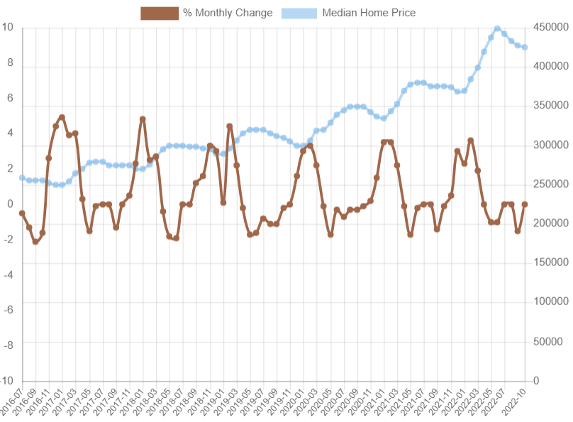
The main image on this preprocessing post shows the true data of median house prices along with their percent change each month. You can click on the legend on top to hide or reveal the % Monthly Change or Median lines:

This chart – which is based upon data available from realtor.com – illustrates a few things. First, that starting in July, 2016 the trend of housing prices clearly rises. Even if we adjust for inflation, the monetary and societal affects of this graph are quite drastic. Second, you can see how aggressively the % Monthly Change tends to rise and fall in a cyclical fashion. When housing prices go up from the previous cycle, the median house price tends to react in the opposite way.

Seeing this true-to-life data visually clues me in right away on a few points:

1. A lot of data needs to be had to try and predict the changes in this chart and its cycles
2. Probably more than time goes into the data changes; forecasting based on time alone is likely not a good approach
3. Even with a great dataset, there are broader global issues at play affecting housing prices

All of these points should be considered when going into a project like this, and any results received from the machine learning model should be used accordingly with that in mind.

Nevertheless, studying the datasets and knowing the true state of things from real-world data gives insight into how complex this problem truly is. Much more could be said and done to get a handle on how to control predictions for such a volatile part of the economy. For now however, we can move on to focus on the datasets and start with the fun cleanup process!

Brace for a Python Code-Walk

It would be best to have the Python code I made specifically for these next steps up while I talk through my decisions. If not, no worries as I’ll also be posting code as I go. I will not cover every single line of Python in the following sections. Instead, I discuss only those code snippets that were created due to a decision I made on preprocessing.

Python Libraries:

I am a fan of scikit-learn due to its ease of use and how intuitive it is for me. We are already clued into the fact that a regression model will be used in some way for the project from Kaggle. Given this, I simply went with scikit-learn libraries to eventually use its linear regression model:

import pandas as pd
import numpy as np
import sklearn.linear_model
from sklearn.metrics import mean_squared_error
import matplotlib.pyplot as plt
from sklearn.preprocessing import OneHotEncoder
from sklearn.preprocessing import LabelEncoder

In addition to these helpful libraries I also brought in the classic pandas, numpy and matplotlib (for a graph toward the end of the code). One item I brought in that isn’t technically used is the LabelEncoder, but I left that in for now since it was helpful in showing me how the categorical variables would be broken up. Feel free to use it for that same purpose as you go, or just take it out altogether otherwise.

Importing and Blending Data:

As usual, I kept things simple by downloading the csv files to my system and pulling them into Python that way. This is not only simple but totally possible given the small size of both sets. The following code accomplishes that, but I also include this here to drive home the point I made earlier on blending both sets together:

housing_train_import = pd.read_csv(wd+'kaggle_train.csv')
housing_test_import = pd.read_csv(wd+'kaggle_test.csv')
df_training = housing_train_import.copy()
df_testing = housing_test_import.copy()
salePrice = df_training['SalePrice']
df_training = df_training.drop('SalePrice',axis=1)
df_training = pd.concat([df_training,df_testing],sort=False).reset_index()

This is all standard stuff, but it is the pd.concat() function that I missed the first time. When running the categorical conversion later on with both sets distinctly, I ran into unique category labels that only existed in one or the other. This wouldn’t be an issue when no category conversion is done. With this project though, since the training set is the one that gets fitted to the regression model, a distinct binary column that only exists in the testing set yields an error when trying to run the model upon it.

This is, therefore, a point worth driving home: combine the datasets for category –> binary conversion.

After combining the sets and then running the OneHot category conversion, my problem was solved, and all columns that needed to exist, existed. This allowed a clean run of the testing set in the regression model.

Data Cleanup:

The next sections of code start with the data cleanup process. This is where reviewing the datasets in step one come in handy. Additionally, I decided to run the following code to understand how many missing or NULL values existed on each column:

for col in df_training:
    print(col,': Missing Percent =',round(df_training[col].isna().sum()/len(df_training),2))

Which revealed the following (Python output is truncated):

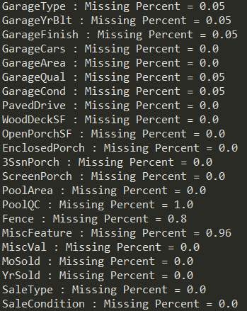
Note in the output what can be seen easily for features ‘PoolQC’, ‘Fence’ and ‘MiscFeature’ which shows all of them missing over 50% of their values. In fact, the other one I chose to omit based on this criteria was ‘Alley’, and so I ran the following on the main dataset:

droppedCols = ['Alley','PoolQC','Fence','MiscFeature']
df_training = df_training.drop(droppedCols,axis=1)

With this step complete I can confidently say that every feature in the data is at least halfway useful. In my real-world experience I come across this type of thing daily. My opinion is such that if the data is trash, send it home. Even if a feature sounds cool and important, if it only is captured on 20% of the data then it will bias your result. I would rather have a solid predictive model without that metric than emotionally trying to fit it in where it only adds the risk of bias. I use the word emotion purposefully here to drive home the point that pragmatism in these types of projects is what matters; we should always guard against personal bias.

Imputing the Numerical Missing Data:

With the dataset containing features that will be kept in the final modeling, it is time to address the missing values. The machine learning model, really any model, won’t handle missing or NULL values. There are several ways to handle this like removing the rows or imputing the data; I tend to favor the latter. Further, I chose imputing because I know I have more than 50% of the data in each feature (see previous section), and thus I make this judgement call from experience and evidence:

for col in df_training:
    if df_training[col].dtypes!='object':
        median = df_training[col].median()
        df_training[col].fillna(median,inplace=True)

It is worth pointing out that in the above loop I am taking advantage of pandas dataframe and its ability to tell me what data type each column is. If it is an object (string) type then I know I can’t calculate a numerical metric upon it. The loop skips these columns and gives the median of only numerical elements. It then adds the established median for that column using the fillna() function and replacing all missing values. I chose median over average to account for outliers, and by the end of the loop I have a clean and properly populated table!

Handling Categorical Missing Data:

Just like the numerical data, categorical features can (and usually will) be missing. This is equally problematic for the future model run and it can be handled by simply populating those columns with anything we like. In this case I chose ‘unknown’ for all missing values in categorical columns:

df_training.fillna('unknown',inplace=True)

Note: I can run this blanket statement against the whole dataset with confidence because I already know the numerical columns are populated. Running this line after the numerical median imputing is non-optional. With that part done, if you want you can rerun the first code from the above data cleanup section and confirm that all features have 0% missing elements now. This is excellent news and right where the data needs to be to move on to the critical data conversion.

OneHotEncoder

Finally, this is the point in which we use the clean dataset to prep for the regression model. As noted earlier, a regression model cannot run using data in a string format. Numbers are required in order to find the best fitting line, regardless of how many dimensions are present in the data.

I like OneHot for a few reasons:

1. It automatically takes the unique values in every column and generates a column for each with a binary reference
2. Approaching the problem in this way avoids the machine learning model from misinterpreting the data in an ordinal way, which wouldn’t make sense

When the process is ran we will go from a 1460 x 81 matrix to 1460 x 335. By combining the testing and training sets upfront we ensure that no unique value on any feature is missed. I split the datasets again into training and testing after this is performed in order to appropriately run the regression.

To accomplish all of this in Python, I call OneHotEncoder():

enc = OneHotEncoder()

With this now assigned to ‘enc’ I can use the fit_transform method on any categorical column and it will automatically create new binary columns on unique values. However, doing this for every categorical feature in the data would be laborious and time-consuming. An important part of programming is to avoid copy & paste type processes. There is almost always a better way!

With this in mind I created the following loop which will call upon the fit_transform method against all categories:

for col in df_training:
    colNames = []
    if df_training[col].dtypes=='object':
      temp = pd.DataFrame(enc.fit_transform(df_training[[col]]).toarray())
      curCol = col
      for col in temp:
        tCol = (curCol+str(col))
        colNames.append(tCol)
      temp.columns = colNames
      df_training = df_training.join(temp)

I am particularly proud of this loop because it took some time to develop carefully and test. However, upon running this in my Python script provided everything will process and add to the dataframe in prep for the final regression run.

I will take a moment to walk through this loop before wrapping up the preprocessing steps for this project. First, note that all processing only takes place on dytpes that equal objects. All numerical features are left alone. Second, once the object column is found I create a temporary dataframe (temp) in which the fit_transform method is applied. We take that column and let OneHotEncoder do its thing, and afterwards pass it to an array. This gets the data in the format I want it in to set up the temporary dataframe, which I eventually add to the training dataset.

The second inner loop is there to add the unique column names to the temporary dataframe. I name every new, unique binary column the original column’s name plus a number in the order for which is was formed. This guarantees that I get a unique name for every new binary column and that no conflicts in creation arise.

Finally, I combine the temp dataframe to the training dataset using the join() function. Once the new binary columns are added to the main dataset, the loop starts again by refreshing the colNames list, hunting for the next object feature, and continuing on. Upon completion, we have a full dataset, with no missing values, categories converted to binary columns, and a few small steps remaining before passing this over to the regression model.

Splitting Datasets

I will not spend too much time on the final stretch of code here simply because it involves only taking out the old categorical columns and splitting the data. It is pretty straightforward compared to everything done through this point.

First, I run this snippet of code to establish the columns I want for the regression:

finalCols = []
for col in df_training:
    if df_training[col].dtypes!='object':
      finalCols.append(col)

By keeping all non-objects in the dataset, we successfully retain our original numerical features along with the new binary columns generated through OneHot.

Importantly, parsing out the testing and training sets into their own dataframes again must be done. Remember that the whole point of this project is to predict the testing values; we also need only the training values to teach the regression model. The following accomplishes splitting the data again by shaving the rows we originally stacked with the concat() function:

df_testing = df_training.iloc[1460:,:].drop('index',axis=1)
df_training = df_training.iloc[0:1460,:].drop('index',axis=1)

Now we have all of the data we wanted and worked for in two distinct datasets! This is where we want to be at this point.

Lastly, we need to take out the IDs that were given to use in the original data since IDs are just there to keep things organized. Additionally, for the regression model, we need to add sale price back into the training set so we have something to predict:

# removing the ids from the datasets
trainingIDs = df_training['Id']
df_training = df_training.drop('Id',axis=1)
testingIDs = df_testing['Id']
df_testing = df_testing.drop('Id',axis=1)
# add back saleprice for the regression model
df_training['SalePrice'] = salePrice

Process Summary

Everything I did in the preprocessing step has been completed. The final testing and training sets are ready for passing into a machine learning model! Since regression is the known method being used that is where the next Python script picks up in the concluding article to this project.

While this post might seem a bit dry to read through it is the heart of what’s necessary to machine learning. The overwhelming effort goes into data preprocessing. If the data going into a model is poorly setup then it is illogical to expect anything other than a poor result. My goal here was to explain in detail my thoughts, reasoning and coding to get a good result on my prediction.

I cover more about how I did in the next post on the housing price regression model. Check out that article next if you’re interested and thanks for reading!

Information References

Real Estate Data. realtor.com. Accessed, 2022-11-27. https://www.realtor.com/research/data/

House Prices – Advanced Regression Techniques. kaggle.com. Accessed, 2022-11-17. https://www.kaggle.com/c/house-prices-advanced-regression-techniques/overview