In this post I chose to cover a topic that I find fascinating: world population. Specifically, what interests me about this topic is how quickly the global population has grown even since I was a kid. Back then, the total world population was 4.6 billion while at present it is over 7.7; this is a 67% increase in under 40 years. If the human population grew this fast throughout history we would already be in an unsustainable state of existence; however, it is not inconceivable to see that the trend as it exists will not slow down. In fact, by 2050 we should be around 9 billion and by 2100 we might hit the 11 billion mark, though there is more to discuss on that prediction.
Regardless, why this topic even matters is a simple question of survival. Not only do we have to contend with the Earth getting warmer we have to deal with more people; that is more mouths to feed, more to shelter and more to hydrate. Water and many other basics of life are already causing problems in the world that will only get worse, but if we understand world population growth and can predict it, then we are better positioned to deal with societal problems that are coming in the future.
Data Gathering and Sourcing
Before getting into the findings from this data I will cover where I sourced it from and how it was manipulated. You can find the data files on my GitHub here. The following files are included for ease of download:
- world_population_data
- life_expectancy
- fertility_rates
- scatter_plot_output
- future_regression_summary
Each of these csv files serve a specific purpose and either contain the data needed within them in order to compare to other metrics or are joined directly together. Additionally, all of the data has been sourced from areas provided at the end of this post.
Visualization Analysis
With the data sourcing elements provided I have provided a few graphs and visual review of code in this post. These are all intended to be thought through in linear terms, meaning, that one idea leads to questions that are answered on the next. As I hear often in the business environment, the concepts here translate into starting at the 30,000 foot view and going down into the data to explain the whys and whats. It is best to keep visuals small & manageable without making 20, 30 or 40 graphs because quantity does not equal good insight.
Population Growth Through 2018 (billions)
We can see in this graph that from 1998 to 2018 there is a linear growth pattern. I can use this data to create a regression line to see if the trend is indeed rising.
What we see is that world population has clearly risen over this timespan. The regression line against all of this data comes out to be:
Population = (92567774 * Year) + (-39573756 * Life Expectancy) + (-176324423234)This regression allows us to predict consequent years into the future with a R2 value of 99%. This taught us two things:
- The trend of world population growth is obvious in that it is rising
- That we need a model with more variables in order to accurately predict this growth velocity
The reason that the R2 value of 99% is both good and bad is because the regression inputs are clearly too simple. We have our time feature (Year), life expectancy and fertility rates included. The regression is dominated by the time component and only takes into account life expectancy as part of a small contribution. The fertility rates do not meet our 95% testing criteria.
The below is a view of what the Python code should have output:
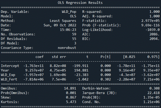
Thanks to the excellent work of the stats model library we can easily analyze this output. You will note that the regression model I gave prior is derived by taking component coefficients from this and applying the y = mx+b formula but with multiple variables. However, the point here on fertility rates is what I wish to highlight and why it isn’t much of a contributor to the model.
Interpreting Model Output
The first place I want to draw attention to is the column header “P>|t|”. Our regression model in Python is defaulting to a 95% confidence level, and thus we want all of the features in this column to be <=5%. This would indicate whether the feature is significantly contributing to the prediction we have made.
Second, the “t” column to the left should be above the absolute value of 2 (written as: |2|) in order to be considered a relevant factor in the model. If these two things are true at the same time then we have proven that they contribute to prediction and are relevant; if the p-value is greater than 5% then we know the “t” column is not relevant and can be dismissed.
Looking through our results with this in mind we see that only the “WLD_Fert” (world fertility rate) is not relevant. It has a p-value of 30% and therefore whatever is shown in the “t” column doesn’t matter. This feature has failed our relevancy test and can be ignored…refer back to the regression model I wrote out to confirm that I have indeed taken it out.
Testing the Regression Model
In the Python script provided there should be an output dataframe that was created called “pop_df”. This was created using the pandas library and contains all of the features discussed so far as well as the predictions the model made. It would look something like this in an IDE (or type pop_df.head() in Python):
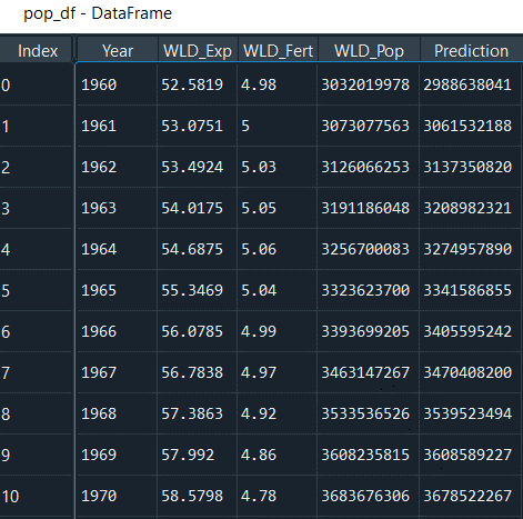
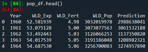
Regardless of how you view the data, we can take the formula given earlier and apply it directly here. Note however that the results from performing the math directly will vary slightly from the dataframe prediction because I have rounded the coefficients for the sake of readability. Even with this slightly different result due to rounding however, we can observe a pretty good predictive model.
Starting with 1960, you can write the prediction out as:
(1960*92567774)+(52.5819*-39573756)+(-176324423234)The resulting world population prediction given this model is: 3,027,550,525. The world population actual at this time was 3,032,019,978 thus given a -0.001 difference in prediction versus actuals; not too bad even with rounding error!
Preparing for Future Predictions
One of the problems here with all the modelling done thus far is that we only really predict past years. The reason for this is because we fed the year and other parameters to the regression based on what already happened; now we are looking to predict values into the unknown.
A Word of Caution: nothing is certain and using a regression model to attempt a view into the future can never be 100% guaranteed.
Let’s take a crack at it anyway to see if we can get some good estimates of world population growth past 2018. We have the benefit of time here because this post is written years after 2018 so we can look back and validate our results. Luckily, the regression model doesn’t know what year it is so we retain this advantage.
We have proven that the world fertility rate is not a contributor to this model. In future posts I will explore this deeper because in truth fertility rates can contribute to population growth and this becomes apparent when we look into more developed countries. However, in this analysis we are looking at aggregate data on the whole and therefore there is information loss when it comes to the nuance that actually exists when we dive deeper.
To continue forward we can use Python to generate a regression formula on year against life expectancy rates. This code is included in the Python script, but for ease of following along here you can process the following code:
modelLE = sm.OLS.from_formula("WLD_Exp ~ Year",data=pop_df)
resultLE = modelLE.fit()
print(resultLE.summary())
From this you would derive the following regression model:
Life Expectancy = (Year*0.3161)+(-564.4153)Plugging into the data we can replace “Year” with 1960 and test how close we get:
(1960*0.3161)+(-564.4153) = 55.14The R2 value on this sub-regression model is 96% and thus we know that 4% of the variance is not explained by the data itself. This is an excellent result regardless and when we compare 55.14 in 1960 against the actual number of 52.58, we see things are not so far off. In 2018 for example the actual life expectancy was 72.6 years old and our regression here predicted 73.5.
With this element in place and our previous regression model already validated, we are ready to put everything together for a basic future-level prediction.
Making a Future Prediction
The next year to predict from the data provided is 2019 and beyond. The further out in time we go the less likely we are to be accurate. This is common sense when thinking about it because the changes in life are always ongoing. This post is written after the 2020 Covid pandemic which certainly skews the data in 2020 and 2021. Hence why I felt it best to look at the aggregate trends in this analysis and dive deeper in future installments on the effects the pandemic had on the trends being revealed here.
The method for performing this prediction is essentially a Python code-walk from here. First, I created a list of the years that I’d like to consider for the future:
yearPredictions = []
x=2018
for i in range(82):
x+=1
yearPredictions.append(x)
Next, we put this list into a dataframe and then call upon the life expectancy sub-regression model to attach those estimates:
pred_df = pd.DataFrame(yearPredictions,columns=['Year'])
pred_df['WLD_Exp'] = (pred_df['Year']*0.3161)+(-564.4153)
At this point in the script, we have a dataframe called “pred_df” which contains all years from 2019 through 2100. The new column ‘WLD_Exp’ was generated using the regression model to establish life expectancy based on the year. With these two features now in existence, the last step is to apply the main regression model to the dataframe:
pred_df['Prediction'] = round((92567774*pred_df['Year'])+(-39573756*pred_df['WLD_Exp'])+(-176324423234),0)That is it! Everything will exist now for the estimates from 2019 – 2100 in the new dataframe. In the Python script referenced throughout this analysis, I do some final steps to stack the original data on top of this new prediction table so that we have one continuous model from which to assess the results. A final snippet of that code is here:
FullLinearPrediction = pop_df.copy()
FullLinearPrediction = FullLinearPrediction[['Year','WLD_Exp','WLD_Pop','Prediction']]
FullLinearPrediction = pd.concat([FullLinearPrediction,pred_df])
With all these steps completed, we could use the ‘FullLinearPrediction’ table to review and analyze our entire model and create some visuals to get a sense of how well we did.
Ending Analysis & Summary
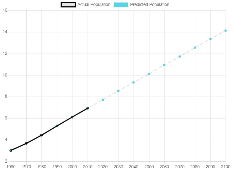
Population Regression Results (in billions)
Based on the full linear prediction table the graph included here shows the actual population versus the predicted number of people starting in 2020. The nice, clean line supports the results we received throughout this entire exercise of a 99% R2 value. If the story stopped here then we would be in great shape having predicted the world’s population growth through to the year 2100.
However, as I noted earlier in the post, there is more to this story. In fact, the linear regression model I’ve created is pretty consistent with the projections made by the U.N. article from 2019 showing that their projection is 9.7 billion people by the year 2050. My regression predicts 10.1 billion or a difference of only 4%! What we need to take into account with all this is the growth of developing countries, better health care around the world, lower fertility rates and a randomness factor (think Covid-19) to adjust this growth accordingly.
It is suggested that the world’s population growth will decline from this trajectory by 2100 and that we will actually be around 11 billion people by then. I tend to agree with this sentiment due to fertility rates dropping and a better quality of life rising around the world, thus leading away from more people having many children. This will be the topic of part two in this analysis where I will dive deeper into individual country statistics, review their quality of life, make predictions and then feed that back into this model. Having done that previously on a different model I already know that the regression calls for around 10-10.5 billion people; around a half-billion short of the U.N. predictions.
I hope that this post was informative and actionable in terms of applying Python regression models to a real-world project. All the code shared here is free to use and leverage for any other analysis you wish to take on. This is a topic that interests me greatly and I will visit it again soon. Thank you for reading and good luck with all your future projects!
Data Source References
The sections below give the source, link and SQL for pulling the data yourself.
Link & SQL for World Population Data
https://console.cloud.google.com/bigquery?utm_source=bqui&utm_medium=link&utm_campaign=classic&project=orion-users&j=bq:US:bquxjob_60129b4b_17da243e7da&page=queryresults
SELECT * FROM bigquery-public-data.world_bank_global_population.population_by_countryLink & SQL for Mortality Rate
https://console.cloud.google.com/bigquery?utm_source=bqui&utm_medium=link&utm_campaign=classic&project=orion-users&j=bq:US:bquxjob_437b9a15_17da2415fd3&page=queryresults
SELECT country_code,year,indicator_name,indicator_code,value
FROM bigquery-public-data.world_bank_health_population.health_nutrition_population WHERE indicator_code ='SP.DYN.LE00.IN' ORDER BY country_code,year
Data Sourcing: Fertility Rates
https://databank.worldbank.org/reports.aspx?source=2&series=SP.DYN.TFRT.IN&country=
Most of this source data was taken from the Google Big Query (GCP) libraries that are offered freely to everyone. With a bit of SQL that I included above and extracting through Python it was easy for me to accomplish the things I needed to with data transformation. The last piece of information was sourced from the World Bank website given that they had the cleanest and most robust fertility rate data that I could trust. Since my data goes as far back as 1960 I needed reliable sources. The data in this analysis therefore starts from 1960 and ends in 2018 given that these years provided the most complete data across the board and allowed me to review everything without making caveats or missing information.
Other References
“Growing at a slower pace, world population is expected to reach 9.7 billion in 2050 and could peak at nearly 11 billion around 2100.” Un.org, 17 Jun. 2019, https://www.un.org/development/desa/en/news/population/world-population-prospects-2019.html